Popular Numbers, Part 3: Matt Parker Breaks the Mould
Welcome to part four in a series examining the popularity of numbers featured in various math resources. Last time, I looked at the popularity of positive rationals on the Numberphile YouTube channel. In this post, I’ll run similar analysis for the standupmaths YouTube channel, a channel where host “[Matt Parker does] mathematics and stand-up. Sometimes simultaneously. Occasionally while being filmed. (It’s quite the Venn diagram.)”.
In the graph below, we can see the popularity of just the standupmaths positive rationals. Because there are only 98 videos, the granularity is too coarse to look at the ratios (as was done previously in the OEIS and Numberphile graphs) – it wouldn’t be clear if the gaps are from the coarse granularity or from a real gap. So we’ll look at raw counts instead of percentages.
source = 'standupmaths'
standupmaths = df_positive_rational[df_positive_rational['source'] == source].copy()
color = colors[source]
plt.scatter(standupmaths.number, standupmaths['count'], marker='.', color=color)
plt.xlabel('Number')
plt.ylabel('Count of videos number occurs in')
plt.title('Popularity of Positive Rationals on standupmaths')
plt.show()
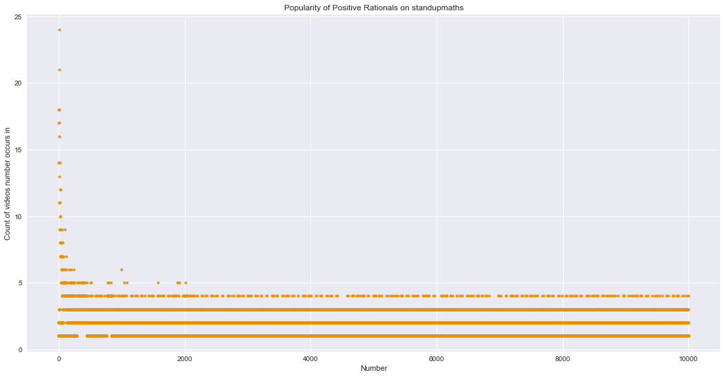
Fascinating! There aren’t any gaps in this data. Unlike OEIS and Numberphile, Matt appears to be an equal-opportunity number enthusiast. Well, except that he also generally favors smaller numbers over larger numbers.
Still, I wonder where the non-integer rationals fall – are they generally less common (as we saw in Numberphile videos)? What about the prime numbers – are they generally more popular (as they were in Numberphile videos and in OEIS)?
standupmaths_nonintegers = standupmaths[standupmaths.number % 1 != 0]
standupmaths_integers = standupmaths[standupmaths.number % 1 == 0].copy()

prior_work_set_names = tag_with_sets_from_prior_work(standupmaths_integers)

standupmaths_primes = standupmaths_integers[standupmaths_integers['primes']]
standupmaths_other = standupmaths_integers[~standupmaths_integers['primes']]
plt.scatter(standupmaths_other.number, standupmaths_other['count'], marker='.', c=plt.cm.Pastel1.colors[0], label='All other numbers')
plt.scatter(standupmaths_nonintegers.number, standupmaths_nonintegers['count'], marker='.', c=plt.cm.Set1.colors[1], label='Non-integers')
plt.scatter(standupmaths_primes.number, standupmaths_primes['count'], marker='.', c=plt.cm.Set1.colors[2], label='Primes')
plt.legend()
plt.xlabel('Number')
plt.ylabel('Count of videos number occurs in')
plt.title('Popularity of Non-Integers and Primes in standupmaths')
plt.show()
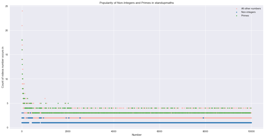
So much for being equal-opportunity number enthusiast. Matt also appears to prefer prime numbers (in green) over non-integers (in blue).
What about the other prior work sets, which generally described popular numbers in the OEIS data by not in the Numberphile data:
- powers: Numbers of the form a^b (for a,b ∈ N)
- squares: Square numbers
- 2^n-1: Numbers one less than a power of 2
- 2^n+1: Numbers one more than a power of 2
- highlyComposites: Guglielmetti defines this as having more divisors than any lower number (i.e. highly composite numbers, see 5040 and other Anti-Prime Numbers)
- manyPrimeFactors: Gauvrit et al. defines this as when “the number of prime factors (with their multiplicty) exceeds the 95th percentile, corresponding to the interval [n − 100, n + 100]”
The graph below shows all of the numbers belonging to these other prior work sets in green compared to the rest of the numbers (in pale red).
standupmaths_integers['unionPriorWorkWithoutPrimes'] = False
for set_name in prior_work_set_names:
    if set_name != 'primes':
        standupmaths_integers['unionPriorWorkWithoutPrimes'] |= standupmaths_integers[set_name]

df_int_others = standupmaths_integers[~standupmaths_integers['unionPriorWorkWithoutPrimes']]
df_int_prior_work_not_primes = standupmaths_integers[standupmaths_integers['unionPriorWorkWithoutPrimes']]

plt.scatter(standupmaths_nonintegers.number, standupmaths_nonintegers['count'], marker='.', c=plt.cm.Pastel1.colors[0], label='Non-integers')
plt.scatter(df_int_others.number, df_int_others['count'], marker='.', c=plt.cm.Pastel1.colors[0], label='All other numbers')
plt.scatter(df_int_prior_work_not_primes.number, df_int_prior_work_not_primes['count'], marker='.', c=plt.cm.Set1.colors[2], label='Prior Work Sets (excl. primes)')
plt.legend()
plt.xlabel('Number')
plt.ylabel('Count of videos number occurs in')
plt.title('Popularity of Prior Work Sets (excluding primes) in standupmaths')
plt.show()
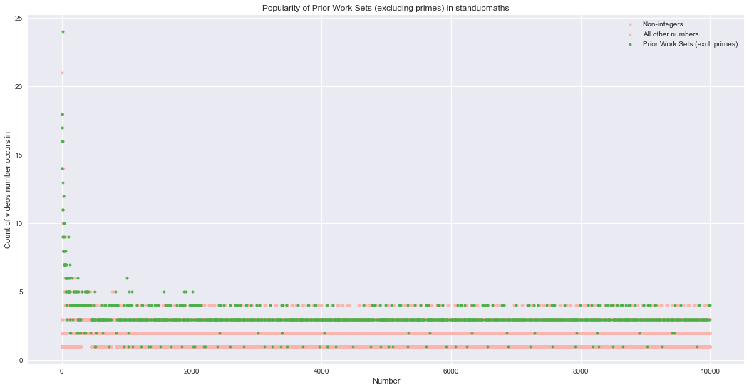
It appears that all of the prior work popular sets are generally good indicators of popularity in standupmaths. So while there isn’t a gap between popularity levels, some sets of numbers still seem to be more popular than others.
The Most Popular
So just who are the most popular positive integers in standupmaths?
standupmaths_sorted = standupmaths.sort_values(by='pct', ascending=False)
tenth_value = standupmaths_sorted.iloc[9].pct
print(standupmaths_sorted[standupmaths_sorted.pct >= tenth_value][['number', 'count', 'pct']])
         number  count       pct
1010857    12.0     24  0.244898
1010257     6.0     21  0.214286
1010020     1.0     18  0.183673
1010157     5.0     18  0.183673
1010024     2.0     18  0.183673
1010657    10.0     17  0.173469
1010057     4.0     17  0.173469
1010457     8.0     16  0.163265
1010357     7.0     16  0.163265
1010002     0.0     14  0.142857
1011657    20.0     14  0.142857
1010051     3.0     14  0.142857
As with OEIS and Numberphile, we again see 1 - 8 are the most popular. Standupmaths also includes zero among the most popular, just like OEIS. Unlike OEIS and Numberphile, 12, 10, and 20 are among the most popular in standupmaths. The numbers aren’t generally in sorted order.
Matt Parker: Venn Diagram Man
Like his channel, Matt Parker is quite the Venn diagram. Not only is he the host on standupmaths, but he’s also the second-most-frequent contributor on Numberphile, hosting 45/359 (12.5%) of videos.
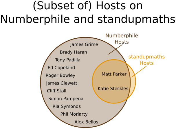
What if we consider combining Matt’s Numberphile videos with his standupmaths videos, since he (presumably) had some say in what numbers were featured in both.
parker = pd.read_sql_query('''SELECT C.real_part AS number, COUNT(*) AS count
                              FROM counts C, hosts H
                              WHERE C.imag_part == 0 AND
                                    C.video_id = H.video_id AND
                                    0 <= C.real_part AND
                                    C.real_part <= 10000 AND
                                    H.host = "Matt Parker"
                              GROUP BY C.real_part''',
                           conn)
df_hosts_counts = pd.read_sql_query('''SELECT H.host, V.source, COUNT(*) AS count
                                       FROM hosts H, videos V
                                       WHERE H.video_id = V.video_id
                                       GROUP BY H.host, V.source''',
                                    conn, index_col='host')
print('How many videos Matt has hosted, by source:\n', df_hosts_counts.loc['Matt Parker'])
total_parker_videos = df_hosts_counts.loc['Matt Parker']['count'].sum()
parker['pct'] = parker.apply(lambda row: row['count']/total_parker_videos, axis=1)
How many videos Matt has hosted, by source:
                    source  count
host
Matt Parker   Numberphile     45
Matt Parker  standupmaths     98
color = '#af6c08'
plt.scatter(parker.number, parker['count'], marker='.', color=color)
plt.xlabel('Number')
plt.ylabel('Count of videos number occurs in')
plt.title('Popularity of Positive Rationals in Videos Hosted by Matt Parker')
plt.show()
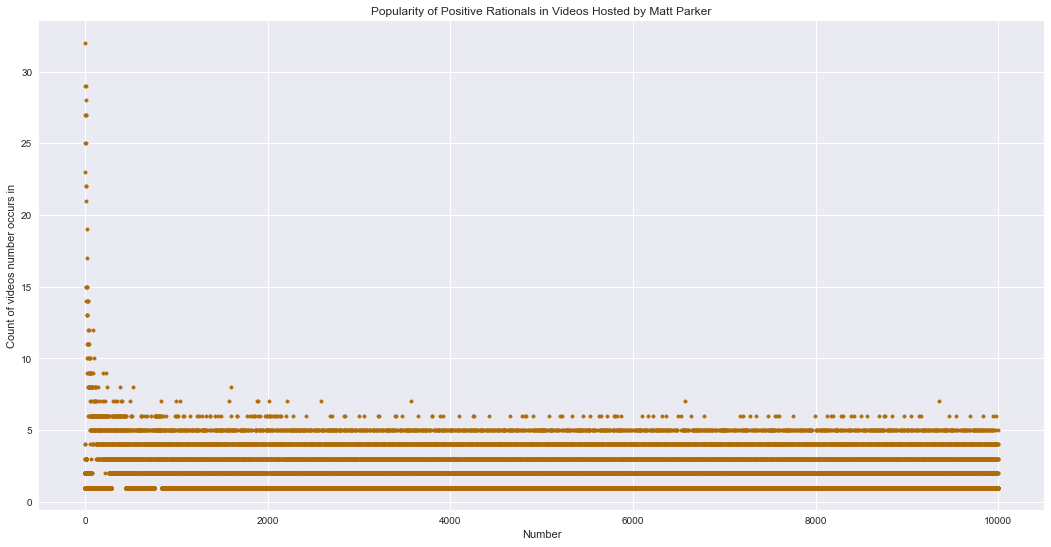
There doesn’t appear to be much of a difference between all the Matt Parker videos and just the standupmaths videos – there’s certainly no obvious gap. Are the most popular numbers also similar?
parker_sorted = parker.sort_values(by='pct', ascending=False)
tenth_value = parker_sorted.iloc[9].pct
print(parker_sorted[parker_sorted.pct >= tenth_value][['number', 'count', 'pct']])
     number  count       pct
25      2.0     32  0.223776
20      1.0     29  0.202797
858    12.0     29  0.202797
258     6.0     28  0.195804
158     5.0     27  0.188811
358     7.0     27  0.188811
52      3.0     27  0.188811
58      4.0     25  0.174825
458     8.0     25  0.174825
0       0.0     23  0.160839
The set of most popular numbers is mostly the same – 10 and 20 dropped off – but the order is different.
A Small Sample Problem?
Compared to OEIS and Numberphile, standupmaths seems to focus on all positive rationals approximately equally. It also has the fewest number of videos – just 98 compared to 359 for all of Numberphile and 296 522 sequences for OEIS. It’s possible that a popularity gap just doesn’t appear when you have a small number of videos. Let’s see if that’s the case.
The graphs below show 98-video/sequence subsets of Numberphile and OEIS data. I try a couple of different subsets:
- The chronologically first 98 Numberphile videos (which includes some hosted by Matt)
- The chronologically first 98 Numberphile videos that weren’t hosted by Matt
- 98 randomly-selected Numberphile videos that weren’t hosted by Matt
- 98 randomly-selected OEIS sequences
- Unfortunately, there’s no simple way to get the first 98 OEIS sequences. From the OEIS page on A-numbers: “When N. J. A. Sloane’s initial collection of sequences reached a few hundred, in the 1960’s, he sorted them in lexicographic order,” then assigned A-numbers in sorted order. Thus, not only are the lower A-numbers not in chronological order, but there’s a bias in the order of those sequences (i.e. they’re likely to contain smaller numbers).
For those randomly-selected subsets, I try a few different random selections, in case there’s anything special about just one random selection. Note that for the OEIS graphs, since they still drop very fast, I show both linear and logarithmic scales on the y-axis.
import time

def reformat_date(d):
    ts = time.strptime(d, '%b %d, %Y')
    return time.strftime('%Y-%m-%d', ts)

def get_counts_by_video_ids(video_ids, df_of_all_numbers=numberphile, df_num_colname='number'):
    video_counts = pd.read_sql_query('''SELECT C.real_part AS number, COUNT(*) AS count
                                        FROM counts C, videos V
                                        WHERE C.imag_part == 0 AND
                                              C.video_id = V.video_id AND
                                              0 <= C.real_part AND
                                              C.real_part <= 10000 AND
                                              V.video_id IN ''' + str(video_ids) + '''
                                        GROUP BY C.real_part''',
                                     conn)
    df_of_all_numbers = df_of_all_numbers[df_num_colname].to_frame()
    video_counts = video_counts.merge(df_of_all_numbers, how='right', on=df_num_colname).fillna(0)
    return video_counts

def get_earliest_k_videos(get_videos_sql, k, df_of_all_numbers=numberphile, df_num_colname='number'):
    video_dates = pd.read_sql_query(get_videos_sql, conn)
    video_dates['iso_date'] = video_dates.date.apply(reformat_date)
    video_dates = video_dates.sort_values(by='iso_date', ascending=True)

    top_k = video_dates.iloc[:k]
    return get_counts_by_video_ids(tuple(top_k.video_id), df_of_all_numbers, df_num_colname)


samples = [('standupmaths', standupmaths, False)]
df = get_earliest_k_videos('''SELECT video_id, date
                              FROM videos
                              WHERE source="Numberphile"''',
                           98)
samples.append(('First 98 Numberphile videos', df, False))

parkerless_np_videos_sql = '''SELECT V1.video_id, V1.date
                              FROM videos V1
                              WHERE V1.source='Numberphile' AND
                                    V1.video_id NOT IN (
                                      SELECT DISTINCT(V2.video_id)
                                      FROM videos V2, hosts H
                                      WHERE V2.source='Numberphile' AND
                                          H.host='Matt Parker' AND
                                          V2.video_id=H.video_id)'''
df = get_earliest_k_videos(parkerless_np_videos_sql, 143)
samples.append(('First 98 Numberphile videos without Matt Parker', df, False))

oeis_a_nums = pd.read_sql_query('SELECT video_id FROM videos WHERE source="OEIS"', conn).video_id
samples_log = []
for i in range(3):
    df = get_counts_by_video_ids(tuple(oeis_a_nums.sample(98, random_state=i)), oeis)
    samples.append(('OEIS Random Subset '+str(i), df, False))
    samples_log.append(('OEIS Random Subset '+str(i)+' logscale', df, True))
samples += samples_log

np_video_ids = pd.read_sql_query(parkerless_np_videos_sql, conn).video_id
for i in range(3):
    df = get_counts_by_video_ids(tuple(np_video_ids.sample(98, random_state=i)))
    samples.append(('Numberphile Random Subset '+str(i)+' without Matt Parker', df, False))
fig, axes = plt.subplots(len(samples)//3, 3, sharex=True)

for i, sample in enumerate(samples):
    row, col = divmod(i, 3)
    ax = axes[row][col]
    title, df, special_plot_type = sample
    if special_plot_type is True:
        ax.semilogy(df.number, df['count'], marker='.', linestyle='')
    else:
        ax.scatter(df.number, df['count'], marker='.')
    if col == 0:
        ax.set_ylabel('# videos number occurs in')
    if row == len(samples):
        ax.set_xlabel('Number')

    ax.set_title(title)

plt.show()
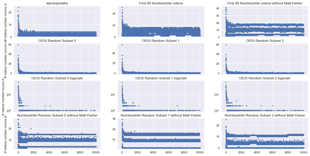
There are some interesting patterns jumping out here. Numberphile appears to have three levels of popularity, even at just 98 videos. However, the distinction between popularity seems to disappear when looking at the first 98 Numberphile videos, including any hosted by Parker. OEIS, however, seems to lose its two levels of popularity. The general popularity of numbers in the OEIS data is also much lower than both Numberphile and standupmaths.
So there definitely appears to be a difference in popularity across the sources, but this post is about standupmaths and Matt Parker, not a comparison of the three sources – that’s another post. So, let’s return to standupmaths. The key takeaway seems to be that even at low sample sizes there could be different levels of popularity. It’s interesting that standupmaths doesn’t seem to have them. In fact, when looking at the first 98 Numberphile videos that include any hosted by Parker, the gaps start disappearing.
Thus it seems that Matt Parker is a “Friend to All Numbers”.
Is “Parker Square” a “Parker Square”?
Matt’s known to not let correctness stand in the way of good math (err, “maths”) fun. He champions, “giving things a go”, even when you don’t exactly succeed [The Parker Square]. Dr. Haran (creator, producer of Numberphile) has coined the term “Parker Square” to describe this phenomena and often uses it to label mistakes. Since “Parker Square” has been coined (in April 2016), have there been more Parker Squares on Numberphile?
import statsmodels.api as sm

import test_facts

filename = 'resources/youtube_facts.py'
facts_lib = test_facts.get_loader_lib(filename)
facts = facts_lib.load_facts()

numberphile_facts = [f for f in facts if f.source == 'Numberphile']
for f in numberphile_facts:
    f.date = reformat_date(f.date)

test_case = test_facts.convert_test_case({'formula' : '1/0'})
parker_squares = [f for f in numberphile_facts if f.test(*test_case)]
assert(len(parker_squares) == len(set([f.link for f in parker_squares])))

all_before_ps = [f for f in numberphile_facts if f.date < '2016-04-18']
n_unique_before = len(set([f.link for f in all_before_ps]))
before_ps = [f for f in parker_squares if f.date < '2016-04-18']
before_ps_pct = len(before_ps) / n_unique_before
print('Errors before "Parker Square" was coined: %d / %d = %0.2f%%' % (len(before_ps), n_unique_before, before_ps_pct*100))

all_after_ps = [f for f in numberphile_facts if f.date > '2016-04-18']
n_unique_after = len(set([f.link for f in all_after_ps]))
after_ps = [f for f in parker_squares if f.date > '2016-04-18']
after_ps_pct = len(before_ps) / n_unique_after
print('Errors after "Parker Square" was coined: %d / %d = %0.2f%%' % (len(after_ps), n_unique_after, after_ps_pct*100))

z_score, p_value = sm.stats.proportions_ztest([len(before_ps), len(after_ps)], [n_unique_before, n_unique_after])
print('p-value =', p_value)
Errors before "Parker Square" was coined: 9 / 274 = 3.28%
Errors after "Parker Square" was coined: 5 / 84 = 10.71%
p-value = 0.269832828101
While the rate of errors shown on Numberphile is over three times greater after “Parker Square” was coined than before, there is no statistically significant difference (at $\alpha$ = 0.05).
What about the hosts with the most errors? Is Mr. Parker the host with the most Parker Squares?
host_counts = {}
for f in parker_squares:
    for h in f.host:
            count = host_counts.get(h, 0)
            count += 1
            host_counts[h] = count

host_occurrences = {}
links_seen = set()
for f in numberphile_facts:
    if f.link in links_seen:
        continue
    links_seen.add(f.link)
    for h in f.host:
        count = host_occurrences.get(h, 0)
        count += 1
        host_occurrences[h] = count

host_freq = {}
for h, c in host_counts.items():
    pct = c / host_occurrences[h] * 100
    print('%s: %d / %d = %0.2f%%' % (h, c, host_occurrences[h], pct)
Matt Parker: 9 / 45 = 20.00%
Cliff Stoll: 2 / 9 = 22.22%
Don Knuth: 1 / 1 = 100.00%
Carlo Séquin: 1 / 5 = 20.00%
Edward Frenkel: 1 / 5 = 20.00%
James Grime: 1 / 82 = 1.22%
Xiaohui Yuan: 1 / 1 = 100.00%
By raw Parker Square count, Matt Parker is quite the Parker Square producer! He’s got 4.5 times the number of Parker Square occurrences as the next guy (Cliff Stoll). Although in his defense, some of those Parker Squares are caused by a calculators he’s unboxing and evaluating (e.g. Calculator Unboxing #6 (Staples collection) and Calculator Unboxing #7 (Gaxio)).
When looking at percent of all occurrences, however, his percentage is about as good as many others. Only James Grime (the most frequent host on Numberphile) has a much lower Parker Square percentage, at just 1.22%.
So depending on how you look at it, Matt is either a prolific Parker Square (at 9 occurrences and counting!) or about average (he does, afterall, host a lot of Numberphile videos). You decide.
Featured Figures and Future Figuring
Some key findings:
- For the most part, Matt treats all positive rationals about equally – there isn’t a popularity gap. However, he does tend to feature non-integers less often than integers, and has a slight focus on the sets of numbers found popular in prior work.
- In Numberphile, errors are not more common after “Parker Square” was coined than before. Additionally, Matt is probably not the greatest source of Parker Squares on Numberphile.