Popular Numbers, Part 2: Numbers on Numberphile
(or, as I’ve been thinking of it: The Point Where it Gets Interesting)
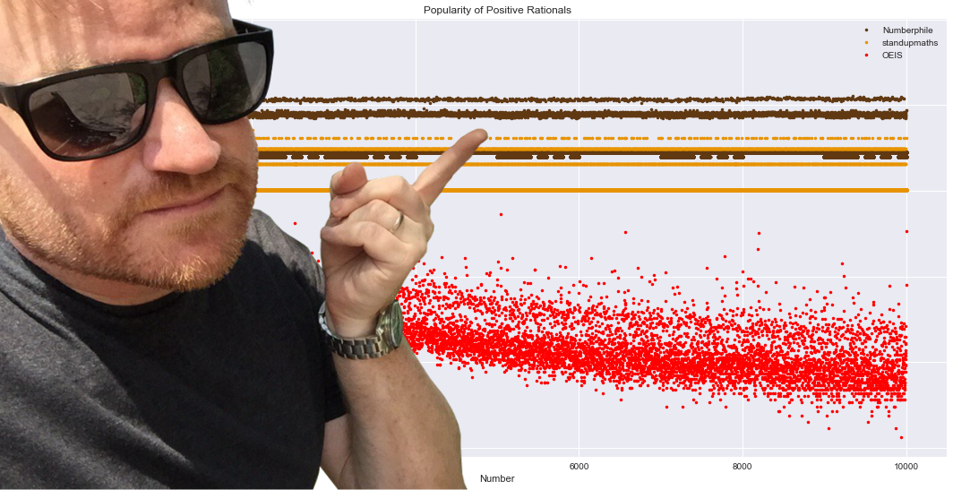
This is the third part in a series examining the popularity of numbers featured in various math resources. Last time, I looked at the popularity of positive integers in OEIS, generally replicating previous work (Guglielmetti and Gauvrit et al.). This time, I’m going to dive into the unexplored realm of the popularity of positive rationals in Numberphile videos, a YouTube channel that’s “Videos about numbers - it’s that simple.”.
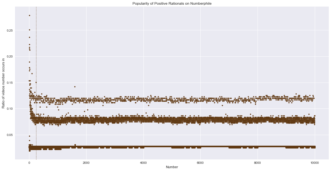
Last time, we saw a graph of positive rational popularity across OEIS, Numberphile, and standupmaths (shown above with Numberphile creator Dr. Haran pointing at the Numberphile data). The graph below is just the popularity of positive rationals in Numberphile.
source = 'Numberphile'
numberphile = df_positive_rational[df_positive_rational['source'] == source].copy()

transition_threshold = 250
color = colors[source]
plt.scatter(numberphile.number, numberphile['pct'], marker='.', color=color)
plt.axvline(x=transition_threshold, linestyle='dotted', color=color, alpha=0.5)
plt.xlabel('Number')
plt.ylabel('Ratio of videos number occurs in')
plt.title('Popularity of Positive Rationals on Numberphile')
plt.show()
Classifying the Popularity
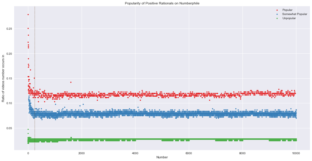
Unlike with the OEIS data, there are very clearly three levels of popularity here: the popular (pct ≈ 0.115), the somewhat popular (pct ≈ 0.078), and the unpopular (pct ≈ 0.025). This is in contrast to OEIS, with only two levels of popularity and a muddy gap between them. However, like OEIS, numbers close to zero are relatively more popular than the line they seem to eventually settle into. I eyeballed the transition point at around number=250 (the dashed line in the graph).
So who’s in each popularity level? First, let’s classify them. For the flat part, a simple kmeans clustering will do. For the curved part, I use two simple thresholds to classify the unpopular (pct <= 0.06) and the obviously popular (pct >= 0.15). For the region between the popular and the somewhat popular, I eyeballed a line that seemed to separate the two (similar to what we did last time for OEIS), going from (12.048, 0.118321) down to (250, 0.0965) – 0.0965 is the average between my initial guesses for the centers of the popular and somewhat popular lines.
from scipy.cluster.vq import kmeans2

estimated_popularity_centers = [0.115, 0.078, 0.025]

threshold_index = numberphile.number[numberphile.number == transition_threshold].index[0]
flat_part = numberphile[threshold_index:]
centroids, flat_groups = kmeans2(flat_part.pct, estimated_popularity_centers)
print('Popularity centers for the flat parts:\n', centroids)

curve_part = numberphile[:threshold_index]

def cluster_curved_Numberphile(row):
    if row.pct <= 0.06:
        return 2
    elif row.pct >= 0.15:
        return 0
    else:
        x1, y1 = 12.048, 0.118321
        x2, y2 = 250, (estimated_popularity_centers[0] + estimated_popularity_centers[1])/2
        m = (y1 - y2) / (x1 - x2)
        b = y1 - m * x1
        if row.pct > m * row.number + b:
            return 0
        else:
            return 1

curve_groups = curve_part.apply(cluster_curved_Numberphile, axis='columns')
numberphile['popularity class'] = np.concatenate([curve_groups, flat_groups])
numberphile['popular'] = numberphile['popularity class'].apply(lambda c: c == 0)

numberphile_popular = numberphile[numberphile['popularity class'] == 0]
numberphile_somewhat_popular = numberphile[numberphile['popularity class'] == 1]
numberphile_unpopular = numberphile[numberphile['popularity class'] == 2]

plt.scatter(numberphile_popular.number, numberphile_popular['pct'], marker='.', color=plt.cm.Set1.colors[0], label='Popular')
plt.scatter(numberphile_somewhat_popular.number, numberphile_somewhat_popular['pct'], marker='.', color=plt.cm.Set1.colors[1], label='Somewhat Popular')
plt.scatter(numberphile_unpopular.number, numberphile_unpopular['pct'], marker='.', color=plt.cm.Set1.colors[2], label='Unpopular')
plt.axvline(x=250, linestyle='dotted', color=color, alpha=0.5)
plt.xlabel('Number')
plt.ylabel('Ratio of videos number occurs in')
plt.title('Popularity of Positive Rationals on Numberphile')
plt.legend()
plt.show()

print('Size of each class:')
for i in range(3):
    print('Class', i)
    popularity_class = numberphile[numberphile['popularity class'] == i]
    size = len(popularity_class)
    print('\tSize:', size)
    print('\tPercent: %0.2f%%' % (100 * size / len(numberphile)))
    print('\tAverage popularity: %0.2f%%' % (100 * popularity_class.mean().pct))
Popularity centers for the flat parts:
 [ 0.11721081  0.07839004  0.02736215]
Size of each class:
Class 0
	Size: 1252
	Percent: 0.13%
	Average popularity: 11.86%
Class 1
	Size: 8749
	Percent: 0.87%
	Average popularity: 7.85%
Class 2
	Size: 990000
	Percent: 99.00%
	Average popularity: 2.73%
Clusters look good. Shockingly, 99% of all the positive rationals studied are unpopular (class 2). What numbers could be so unpopular?
Characterizing the Unpopular Numbers
I strongly suspect that all the non-integers are in this category since 990000 is exactly how many positive non-integer rationals are included in the analysis.
numberphile_nonintegers = numberphile[numberphile.number % 1 != 0]
print('Classes that non-integers appear in:', numberphile_nonintegers['popularity class'].unique())
print('Total number of non-integers:', len(numberphile_nonintegers))
Classes that non-integers appear in: [2]
Total number of non-integers: 990000
Yep, the unpopular numbers are all the non-integers. With an average popularity of 2.74%, they are only a quarter as popular as the popular numbers and less than half as popular as the somewhat popular numbers. On average, they’re featured in only about 10 Numberphile videos so far. Sorry non-integers, but at least you’re still interesting.
The distribution of popularity among the unpopular numbers is:
numberphile_unpopular_counts = numberphile_unpopular.groupby('pct').pct.count()
plt.stem(numberphile_unpopular_counts.index.values, numberphile_unpopular_counts.values)
for x, y in numberphile_unpopular_counts.items():
    plt.annotate(y, xy=(x, y+10000), ha='center')

plt.xticks(numberphile_unpopular_counts.index.values)
plt.xlabel('Percent of videos')
plt.ylabel('# of non-integers')
plt.title('Distribution of Popularity among Unpopular Positive Rationals in Numberphile')
plt.show()
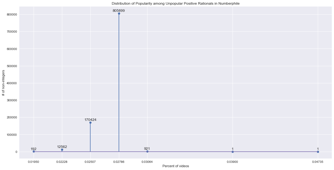
Most of the non-integers are between 2.2284% and 2.7855%. A small but sizeable percentage of numbers occur in only 1.95% of videos (7 videos) and a larger percentage occurring in 3.06% of videos (11 videos). Interestingly, there are two positive non-integers even higher.
numberphile_unpopular[numberphile_unpopular.pct > 0.035]
| source | number | count | pct | popularity class | popular | |
|---|---|---|---|---|---|---|
| 25 | Numberphile | 0.25 | 14 | 0.038997 | 2 | False |
| 50 | Numberphile | 0.50 | 17 | 0.047354 | 2 | False |
The powers of two! Powers of two have been observed in the OEIS data to be popular (“La minéralisation des nombres” by Guglielmetti and in the previous post of this series) and here we see that even the negative powers of two continue the trend of being popular. Later in the series, we’ll take a closer look at the trend of powers of two.
I’m surprised we didn’t see any approximations of popular constants (e.g. 3.14 for pi) pop out among the most popular non-integers. Later in the series we’ll focus on regions around popular constants. For now, let’s move on.
Characterizing the Popular Numbers
Now that we know what the unpopular numbers are, let’s figure out who some of the popular numbers are. For this analysis, I’ll look just at the integers since we already know that all the non-integers are unpopular. Last time, I drew from previous work by Guglielmetti and Gauvrit et al. to create sets of likely-popular numbers:
- primes: Prime numbers
- powers: Numbers of the form a^b (for a,b ∈ N)
- squares: Square numbers
- 2^n-1: Numbers one less than a power of 2
- 2^n+1: Numbers one more than a power of 2
- highlyComposites: Guglielmetti defines this as having more divisors than any lower number (i.e. highly composite numbers, see 5040 and other Anti-Prime Numbers)
- manyPrimeFactors: Gauvrit et al. defines this as when “the number of prime factors (with their multiplicty) exceeds the 95th percentile, corresponding to the interval [n − 100, n + 100]”
Last time, I also generated a set that’s the union of those above, named unionPriorWork.
In general, these turned out to be useful sets, so I’ll try them again. Luckily, I also created a function that’ll do the tagging for us: tag_with_sets_from_prior_work!
numberphile_ints = numberphile[numberphile.number % 1 == 0].copy()
prior_work_set_names = tag_with_sets_from_prior_work(numberphile_ints)
numberphile_class_metrics = get_classification_metrics_for_all_prediction_labels(numberphile_ints, 'popular', prior_work_set_names)
render_classification_metrics_table(numberphile_class_metrics, True)
| predictor | precision | recall | f1 | # predicted |
|---|---|---|---|---|
| primes | 1.00 | 0.98 | 0.99 | 1229 |
| unionPriorWork | 0.72 | 0.99 | 0.83 | 1719 |
| 2^n-1 | 0.54 | 0.01 | 0.01 | 13 |
| 2^n+1 | 0.38 | 0.00 | 0.01 | 13 |
| squares | 0.05 | 0.00 | 0.01 | 100 |
| powers | 0.04 | 0.00 | 0.01 | 124 |
| highlyComposites | 0.22 | 0.00 | 0.01 | 18 |
| manyPrimeFactors | 0.00 | 0.00 | 0.00 | 370 |
The table above shows various metrics for each set. As in the previous post, the table is sorted by f1 and the metrics cells are color-coded by how high their value is (white -> 0, blue -> 1) – higher is better.
Here’s where it gets interesting! Two findings immediately jump out. First, only the primes seem to do a great job of predicting popularity, with perfect precision and almost perfect recall (at 0.98). The union of all the sets does a fairly good job with 0.72 precision and 0.99 recall. The rest don’t have very good precision and have horrible recall.
This brings me to the second finding. With the exception of primes and probably unionPriorWork, these sets are horrible at predicting popularity in the Numberphile positive integers. For the OEIS positive integers, they were actually fairly good. The worst precision there (manyPrimeFactors, 0.65) is better than all but two of the precisions here. Similarly, for each set the recall here is worse than the recall in the OEIS data (except for primes and unionPriorWork).
Notice that of the 1252 popular numbers on Numberphile, 1229 of them are prime (98.2%). Given this finding, I propose the Numberphile Primality Test: If a number occurs frequently on Numberphile, then it’s probably prime, with 98.2% probability.
The Non-Prime Popular Numbers
There are, however, 23 popular positive integers that aren’t prime. What are those?
numberphile_popular = numberphile_ints[numberphile_ints.popular]
numberphile_popular_nonprimes = numberphile_popular[~numberphile_popular.primes]
numberphile_popular_nonprimes_nums = [int(n) for n in numberphile_popular_nonprimes.number]
print('Non-prime popular positive integers in Numberphile:')
print(numberphile_popular_nonprimes_nums)
Non-prime popular positive integers in Numberphile:
[0, 1, 4, 6, 8, 9, 10, 12, 14, 15, 16, 18, 20, 21, 34, 55, 144, 377, 610, 987, 2584, 4181, 6765]
All of the non-primes in the range [0, 21] are popular; this is consistent with OEIS.
Notice that even including all sets, we get a recall of 0.99 – close, but not perfect. It’s higher than the recall of just the primes set, so some of those non-primes are covered by other sets. Which popular numbers are false negatives (i.e. aren’t included in any of the sets)?
numberphile_popular_accounted = numberphile_popular[numberphile_popular.unionPriorWork]
numberphile_popular_unaccounted = numberphile_popular[~numberphile_popular.unionPriorWork]

print('Unaccounted:')
print([int(n) for n in numberphile_popular_unaccounted.number])
Unaccounted:
[6, 10, 14, 18, 20, 21, 34, 55, 377, 610, 987, 2584, 4181, 6765]
So nine non-primes were covered by the other sets, leaving 14 popular numbers unaccounted for. The graph below shows where those popular numbers fall within the Numberphile popularity graph.
plt.scatter(numberphile_popular.number, numberphile_popular['pct'], marker='.', color=plt.cm.Pastel1.colors[0], label='Popular')
plt.scatter(numberphile_somewhat_popular.number, numberphile_somewhat_popular['pct'], marker='.', color=plt.cm.Pastel1.colors[1], label='Somewhat Popular')
plt.scatter(numberphile_unpopular.number, numberphile_unpopular['pct'], marker='.', color=plt.cm.Pastel1.colors[2], label='Unpopular')
plt.scatter(numberphile_popular_unaccounted.number, numberphile_popular_unaccounted['pct'], marker='.', color=plt.cm.Set1.colors[0], label='Unaccounted For Popular')
plt.axvline(x=250, linestyle='dotted', color=color, alpha=0.5, label='Curve->Flat Threshold')
plt.legend()
plt.xlabel('Number')
plt.ylabel('Ratio of videos number occurs in')
plt.title('Non-Prime Popular Numbers in Numberphile Positive Integers')
plt.show()
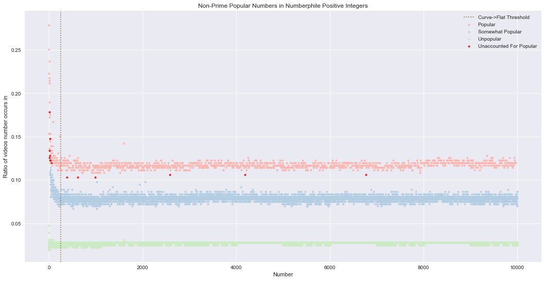
It seems many of them occur for smaller numbers, before the curves level out (the dashed brown line). For the ones in the flat part, it looks like all of the non-prime populars are the least popular of the popular. Just to confirm, below I look at the six least popular of the popular numbers. They should match the last six in the list of non-prime popular positive integers shown above.
print('Least popular of the popular numbers:')
display(HTML(numberphile_popular.sort_values(by='pct', ascending=True)[['number', 'pct']].iloc[:6].to_html(index=False)))
Least popular of the popular numbers:
| number | pct |
|---|---|
| 610.0 | 0.103064 |
| 377.0 | 0.103064 |
| 987.0 | 0.103064 |
| 6765.0 | 0.105850 |
| 4181.0 | 0.105850 |
| 2584.0 | 0.105850 |
Yes, they’re a match! How close is the next least-popular of the popular integers is?
numberphile_popular.sort_values(by='pct', ascending=True)[['number', 'pct']].iloc[6]
number    919.000000
pct         0.108635
Name: 91900, dtype: float64
It turns out that there’s a difference of 2.785 percentage points between those six unaccounted for “popular” numbers and the accounted for ones. Perhaps this means the clustering algorithm picked a poor threshold. However, they do look closer to the popular numbers than the semipopular numbers, so maybe they’re popular but don’t fall into any of those sets. I wonder if they’re popular in OEIS.
numberphile_popular_unaccounted_over_376 = numberphile_popular_unaccounted[numberphile_popular_unaccounted.number > 376]
numberphile_unaccounted_intersect_oeis = oeis_popular[oeis_popular.number.isin(numberphile_popular_unaccounted_over_376.number)]
print('Unaccounted for popular Numberphile numbers that are also popular in OEIS:')
print(numberphile_unaccounted_intersect_oeis.number.values)
Unaccounted for popular Numberphile numbers that are also popular in OEIS:
[ 2584.  4181.  6765.]
So the three larger numbers were popular in OEIS, but the other half weren’t. At this time, it’s unclear what makes them popular.
The Most Popular
So just who are the most popular positive integers in Numberphile?
numberphile_sorted = numberphile.sort_values(by='pct', ascending=False)
tenth_value = numberphile_sorted.iloc[9].pct
print(numberphile_sorted[numberphile_sorted.pct >= tenth_value][['number', 'count', 'pct']])
      number  count       pct
300      3.0    100  0.278552
200      2.0     90  0.250696
500      5.0     85  0.236769
100      1.0     80  0.222841
400      4.0     78  0.217270
700      7.0     77  0.214485
1300    13.0     76  0.211699
800      8.0     68  0.189415
600      6.0     64  0.178273
1700    17.0     63  0.175487
As with the OEIS data, numbers 1 - 8 are in the top ten most popular, but that’s about where the similarity ends. OEIS included 0 and 9, but Numberphile has 13 and 17 instead perhaps because of Numberphile’s greater focus on primes (as discovered above). It’s also interesting that the numbers aren’t mostly in sorted order like they were with OEIS.
Featured Figures and Future Figuring
Some key findings:
- There are three popularity classes:
- Popular: averaging 11.7% of videos, consist almost exclusively of prime numbers
- Semipopular: averaging 7.84% of videos, consists of all integers that aren’t popular
- Unpopular: averaging 2.74% of videos, consisting of all non-integers
- Dr. Haran, what do you have against the non-integers?
- Other than primes, none of the sets identified in previous work are good at predicting popularity in Numberphile videos
It’s important to keep in mind the potential flaws in the data collection/annotation, which can bias the findings presented above:
- the data was collected to display facts in a child’s calculator
- there was only one annotator