Popular Numbers, Part 1: Popularity of Positive Rationals in OEIS
In this series, we’re looking at the popularity of numbers in various online math resources. Previously, I reviewed the data being used in this analysis. In this part, I’ll finally start doing some analysis! I’ll start with a quick overview of the popularity of numbers across the sources, then I’ll dive into the OEIS data by trying to replicate the results in the Sloane’s Gap paper (Numberphile video on the topic).
Loading Data
Let’s assume that the scripts from https://github.com/lipschultz/diabicus/blob/gap-analysis/number-analysis/ have been used to save the data into a database. First I load all the positive rational data.
import sqlite3
import pandas as pd

conn = sqlite3.connect('data/data.db')
df_positive_rational = pd.read_sql_query('''SELECT V.source, C.real_part AS number, COUNT(*) AS count
                                            FROM counts C, videos V
                                            WHERE C.imag_part == 0 AND
                                                  C.video_id = V.video_id AND
                                                  0 <= C.real_part AND
                                                  C.real_part <= 10000
                                            GROUP BY V.source, C.real_part''',
                                         conn)
Each source has a different number of videos/sequences, from 98 with standupmaths to 296 522 with OEIS. Brady, Matt: if you just increase your output to about 81 videos/day, you should be able to catch up in only 10 years – get on it! (please). In the meantime, I need to normalize by the number of videos/sequences, which the code below does (saving it in a new column named pct).
df_source = pd.read_sql_query('''SELECT source, COUNT(*) as total
                                 FROM videos
                                 GROUP BY source''',
                              conn, index_col='source')
source_totals = df_source['total'].to_dict()
df_positive_rational['pct'] = df_positive_rational.apply(lambda row: row['count']/source_totals[row['source']], axis=1)
Qualitative Comparison of Sources
With the data loaded, I couldn’t wait to see what the popularities look like!
import matplotlib.pyplot as plt
import seaborn as sns
%matplotlib inline
sns.set()
plt.rcParams["figure.figsize"] = (18, 9)

colors = {'Numberphile': '#603913', 'standupmaths': '#e79300', 'OEIS': '#ff0000'}

for source, color in colors.items():
    d = df_positive_rational[df_positive_rational['source'] == source]
    plt.semilogy(d.number, d['pct'], marker='.', linestyle='', label=source, color=color)

plt.legend()
plt.xlabel('Number')
plt.ylabel('Ratio of videos number occurs in')
plt.title('Popularity of Positive Rationals')
plt.show()

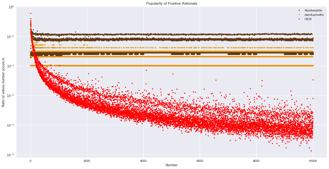
The graph above shows OEIS popularity in red, standupmaths in yellow, and Numberphile in brown. The y-axis is logscale. A few interesting things pop out.
The Numberphile and standupmaths plots are mostly straight lines, with a slight curve close to zero. This is in stark contrast with OEIS, which has a general downward trend throughout the graph. OEIS might be different because of their length threshold on each sequence – bigger numbers may be dropped and longer sequences truncated. However, there may be fundamental differences between OEIS and the two YouTube channels. The people who decide what numbers/sequences to include are different (OEIS has a panel of mathematicians, Numberphile has Dr. Haran and mathematicians, standupmaths has Matt Parker and his guests), possibly leading to different focuses. Of course, I also annotated the YouTube data (and didn’t have a second annotator), so this difference might be my fault.
Both Numberphile and standupmaths have very clearly-defined gaps compared to OEIS. This might be due to just having less videos than OEIS has sequences: more sequences leads to finer granularity between 0% and 100%, allowing for a muddier gap. Having more sequences also allows for less popular sequences (e.g. OEIS keywords “dumb”, “less”, or “obsc”), which Numberphile and standupmaths maybe haven’t gotten to (yet?). The same reasons in the previous paragraph could also apply here.
Finally, almost all OEIS data points are below the other two sources. This is likely because there are just more sequences in OEIS than videos in Numberphile and standupmaths, and each number just shows up in a small percentage of those sequences.
Now let’s dive into the details of the specific curves, starting with OEIS!
Positive Integers in OEIS
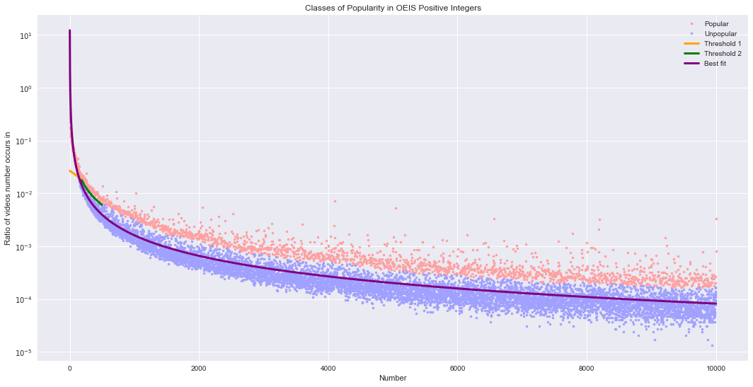
In the graph above, notice that the OEIS data is similar to Figure 1 from the Sloane’s Gap paper, which we’d expect since the data is largely identical. While there is still a noticeable gap, it is less pronounced than in the Sloane’s Gap paper. I suspect the difference is in how we counted occurrences: they count all occurrences of a number, while I counted the sequences a number appears in.
Curve
The general downward trend of the popularity appears to be a logarithmic curve (as was used in the Sloane’s Gap paper). Fitting a logarithmic curve to the data shows that it is a good fit:
import numpy as np
from scipy import stats

oeis = df_positive_rational[df_positive_rational['source'] == 'OEIS'].copy()

oeis_regression = stats.linregress(np.log(oeis.number[1:]), np.log(oeis['pct'][1:]))
print('OEIS regression:', oeis_regression)
print()
print('popularity = %f * n^%f' % (np.exp(oeis_regression.intercept), oeis_regression.slope))
oeis_best_fit = lambda n: np.exp(oeis_regression.intercept) * n**oeis_regression.slope
OEIS regression: LinregressResult(slope=-1.2936573821919723, intercept=2.5035990376186987, rvalue=-0.91845336952248591, pvalue=0.0, stderr=0.0055716551335381085)

popularity = 12.226418 * n^-1.293657
The curve is a very good fit at p ≈ 0.0 and r^2 = 0.84 (compared to r^2 = 0.81 in the Sloane’s Gap paper). The slope/exponent is also very similar to the one found in Sloane’s Gap paper (exponent = -1.33).
Classifying the Popular Numbers
As with the Sloane’s Gap paper, I’ll empirically determine which numbers are popular. Two curves will determine popularity for the regions [0, 185) and [185, 500). For 500 and above, I use the same method as Gauvrit et al.: numbers with a popularity above the 82 percentile within the range [n-c, n+c] are labeled popular; for n <= 1000, c = 100, for n > 1000, c = 350.
from collections import namedtuple

Point = namedtuple('Point', ['x', 'y'])

def line_from_points(point1, point2):
    m = (point1.y - point2.y) / (point1.x - point2.x)
    b = point1.y - m*point1.x
    return m, b

point1 = Point(100, 0.0219296)
point2 = Point(185, 0.0178644)
m1, b1 = line_from_points(point1, point2)
threshold_curve1 = lambda x: m1 * x + b1

point3 = Point(499, 0.00609301)
point2log = Point(*[np.log(p) for p in point2])
point3log = Point(*[np.log(p) for p in point3])
m2, b2 = line_from_points(point2log, point3log)
threshold_curve2 = lambda x: np.exp(b2 + m2 * np.log(x))

is_popular = []
for i in range(len(oeis)):
    number = oeis.iloc[i]['number']
    pct = oeis.iloc[i]['pct']
    if number < 185:
        is_popular.append(pct > threshold_curve1(number))
    elif number < 500:
        is_popular.append(pct > threshold_curve2(number))
    else:
        window_size = 100 if number <= 1000 else 350
        lower_bound = max(0, i-window_size)
        upper_bound = min(i+window_size, len(oeis)-1)
        interval = oeis.iloc[lower_bound:upper_bound+1]
        threshold_pct = interval['pct'].quantile(0.82)
        is_popular.append(pct > threshold_pct)

oeis['popular'] = is_popular
The figure below shows the classified numbers, the two threshold curves, as well as the line of best fit for all the data. We also see that there are 1964 positive integers in the popular set, 19.6% of all positive integers considered.
oeis_popular = oeis[oeis.popular]
oeis_regular = oeis[~oeis.popular]

print('Number of popular integers:', len(oeis_popular))
print('Number of unpopular integers:', len(oeis_regular))

plt.semilogy(oeis_popular.number, oeis_popular['pct'], label='Popular', c='#ffa0a0', marker='.', linestyle='')
plt.semilogy(oeis_regular.number, oeis_regular['pct'], label='Unpopular', c='#a0a0ff', marker='.', linestyle='')
x_1 = [x for x in range(0, 185)]
plt.semilogy(x_1, [threshold_curve1(x) for x in x_1], label='Threshold 1', c='orange', marker='', linestyle='-', linewidth=3)
x_2 = [x for x in range(185, 500)]
plt.semilogy(x_2, [threshold_curve2(x) for x in x_2], label='Threshold 2', c='green', marker='', linestyle='-', linewidth=3)
plt.semilogy(oeis.number[1:], oeis.number[1:].apply(oeis_best_fit), label='Best fit', c='purple', marker='', linestyle='-', linewidth=3)
plt.legend()
plt.xlabel('Number')
plt.ylabel('Ratio of videos number occurs in')
plt.title('Classes of Popularity in OEIS Positive Integers')
plt.show()
Number of popular integers: 1964
Number of unpopular integers: 8037

Characterizing the Popular Numbers
Now that we’ve classified the numbers, let’s find out who’s in the popular class.
Prior work by Guglielmetti and Gauvrit et al. found that the popular positive integers tend to belong to one or more of these sets:
- primes: Prime numbers
- powers: Numbers of the form a^b (for a,b ∈ N)
- squares: Square numbers
- 2^n-1: Numbers one less than a power of 2
- 2^n+1: Numbers one more than a power of 2
- highlyComposites: Guglielmetti defines this as having more divisors than any lower number (i.e. highly composite numbers, see 5040 and other Anti-Prime Numbers)
- manyPrimeFactors: Gauvrit et al. defines this as when “the number of prime factors (with their multiplicty) exceeds the 95th percentile, corresponding to the interval [n − 100, n + 100]”
The code below tags each number for whether it belongs to one of those seven sets. It also creates a new set that’s the union of the sets above: unionPriorWork.
import sys
sys.path.append('../src')
import numeric_tools


def get_powers_of(base, starting_exponent=2, no_values_above=10000):
    values = []
    exponent = starting_exponent
    value = base ** exponent
    while value <= no_values_above:
        values.append(value)
        exponent += 1
        value = base ** exponent
    return values

def tag_with_prime_set(df):
    df['primes'] = df.number.apply(numeric_tools.is_prime)
    return ['primes']

def tag_with_powers(df, max_num, *, do_power=True, do_square=True, do_power_2_less_1=True, do_power_2_plus_1=True):
    set_names = []

    powers = set()
    squares = [1] # To be consistent with Guglielmetti, who includes 1
    base = 2
    base_powers = get_powers_of(base, no_values_above=max_num)
    powers_of_2 = [1] + base_powers
    while len(base_powers) > 0:
        powers.update(base_powers)
        squares.append(base_powers[0])
        base += 1
        base_powers = get_powers_of(base, no_values_above=max_num)

    if do_power:
        df['powers'] = df.number.apply(lambda n: n in powers)
        set_names.append('powers')

    if do_square:
        df['squares'] = df.number.apply(lambda n: n in squares)
        set_names.append('squares')

    if do_power_2_less_1:
        one_less_than_power_of_two = [n - 1 for n in powers_of_2]
        df['2^n-1'] = df.number.apply(lambda n: n in one_less_than_power_of_two)
        set_names.append('2^n-1')

    if do_power_2_plus_1:
        one_more_than_power_of_two = [n + 1 for n in powers_of_2]
        df['2^n+1'] = df.number.apply(lambda n: n in one_more_than_power_of_two)
        set_names.append('2^n+1')

    return set_names

def tag_with_highly_composite(df, max_num):
    more_divisors_than_predecessors = [1] # To be consistent with Guglielmetti, who includes 1
    max_divisor_count = 1
    n = 2
    while n <= max_num:
        divisor_count = len(numeric_tools.factors(n, numeric_tools.FACTORS_ALL))
        if divisor_count > max_divisor_count:
            more_divisors_than_predecessors.append(n)
            max_divisor_count = divisor_count
        n += 1
    df['highlyComposites'] = df.number.apply(lambda n: n in more_divisors_than_predecessors)
    return ['highlyComposites']

def tag_with_many_prime_factors(df):
    df['prime_factor_count'] = df.number.apply(lambda n: len(numeric_tools.factors(n, numeric_tools.FACTORS_PRIME)))
    has_many_prime_factors = []
    for i in range(len(df)):
        lower_bound = max(0, i-100)
        upper_bound = min(i+100, len(df)-1)
        interval = df.iloc[lower_bound:upper_bound+1]
        threshold_95pct = interval.prime_factor_count.quantile(0.95)
        has_many_prime_factors.append(df.iloc[i].prime_factor_count > threshold_95pct)
    df['manyPrimeFactors'] = has_many_prime_factors
    return ['manyPrimeFactors']

def tag_with_sets_from_prior_work(df):
    MAX_NUMBER = df.number.max()
    set_names = []

    set_names.extend(tag_with_prime_set(df))
    set_names.extend(tag_with_powers(df, MAX_NUMBER))
    set_names.extend(tag_with_highly_composite(df, MAX_NUMBER))
    set_names.extend(tag_with_many_prime_factors(df))

    df['unionPriorWork'] = False
    for set_name in set_names:
        df['unionPriorWork'] |= df[set_name]
    set_names.append('unionPriorWork')
    return set_names


prior_work_set_names = tag_with_sets_from_prior_work(oeis)
oeis['popularity class'] = oeis.popular
Now let’s look at the results!
Let’s consider each of the sets as a classifier – if a number belongs to the set, then it’s predicted to belong to the popular class. With this view, the authors of the Sloane’s Gap paper report precision and recall for primes, squares, and manyPrimeFactors. They additionally report the negative predictive value for the primes, and false omission rate for squares and manyPrimeFactors. They don’t report metrics for any of the other sets and the metrics they report are for numbers in the range [301, 10000]. Below, I do some setup to compute the metrics, then report on all of the sets and compute the metrics for numbers in the range [0, 10000].
from sklearn.metrics import confusion_matrix, precision_score, recall_score, f1_score
from IPython.core.display import display, HTML

def get_classification_metrics(df, true_label, pred_label):
    class_values = list(set(df[pred_label].unique()) | set(df[true_label].unique()))
    class_values.sort()

    tn, fp, fn, tp = confusion_matrix(df[true_label], df[pred_label]).ravel()

    metrics = pd.DataFrame({'predictor': [pred_label]*len(class_values),
                            'class': class_values})
    metrics['precision'] = precision_score(df[true_label], df[pred_label], average=None)
    metrics['recall'] = recall_score(df[true_label], df[pred_label], average=None)
    metrics['f1'] = f1_score(df[true_label], df[pred_label], average=None)
    if len(class_values) == 2:
        p = list(metrics['precision'])
        p.reverse()
        #metrics['negative predictive value'] = p
        #metrics['false omission rate'] = [1-v for v in p]
    metrics['# predicted'] = oeis.groupby(pred_label).count().ix[:, 0].values
    return metrics

def get_classification_metrics_for_all_prediction_labels(df, true_label, pred_label_list):
    metrics = pd.DataFrame()
    for set_name in prior_work_set_names:
        metrics = metrics.append(get_classification_metrics(df, true_label, set_name))
    return metrics

def render_classification_metrics_table(metrics, for_class, sort_by='f1', do_not_color=['predictor', '# predicted']):
    class_metrics = metrics[metrics['class'] == for_class].drop('class', 1)
    class_metrics = class_metrics.sort_values(by=sort_by, ascending=False)

    cmap = sns.light_palette("blue", as_cmap=True)
    to_hexcolor = lambda val: '#' + ''.join(['%02x' % int(v*255) for v in cmap(int(val*255))[:-1]])

    rows = ['<th>' + '</th><th>'.join(class_metrics.columns.tolist()) + '</th>']
    for i, row in class_metrics.iterrows():
        cells = []
        for col_name, val in row.items():
            style = 'text-align:center;'
            if col_name not in do_not_color:
                style += 'background-color:{color};'.format(color=to_hexcolor(val))
                if val > 0.5:
                    style += 'color:white;'
            if not isinstance(val, str) and (0 <= val <= 1):
                val = '%0.02f' % val
            cell = '<td style="{style}">{value}</td>'.format(style=style, value=val)
            cells.append(cell)
        rows.append(''.join(cells))

    rendered_rows = '<tr>' + '</tr><tr>'.join(rows) + '</tr>'
    display(HTML('<table>' + rendered_rows + '</table>'))

oeis_class_metrics = get_classification_metrics_for_all_prediction_labels(oeis, 'popularity class', prior_work_set_names)
render_classification_metrics_table(oeis_class_metrics, True)
| predictor | precision | recall | f1 | # predicted |
|---|---|---|---|---|
| unionPriorWork | 0.91 | 0.79 | 0.84 | 1719 |
| primes | 0.98 | 0.61 | 0.75 | 1229 |
| manyPrimeFactors | 0.65 | 0.12 | 0.21 | 370 |
| powers | 0.94 | 0.06 | 0.11 | 124 |
| squares | 0.94 | 0.05 | 0.09 | 100 |
| highlyComposites | 1.00 | 0.01 | 0.02 | 18 |
| 2^n-1 | 1.00 | 0.01 | 0.01 | 13 |
| is_2^n+1 | 0.92 | 0.01 | 0.01 | 13 |
The table above shows various metrics for each set. The table is sorted by f1 and the metrics cells are color-coded by how high their value is (white -> 0, blue -> 1) – higher is better.
We see that these sets generally have very good precision. Only manyPrimeFactors has a precision below 0.90, at 0.65. This is consistent with the Sloane’s Gap paper, where they also found very good precision for primes and squares, but poorer precision for having many prime factors. However, the best precision comes from two sets the authors brushed over, highlyComposite and 2^n-1, with perfect precision.
Unfortunately, the high precision generally comes at very low recall. Most of these sets are small, generally being less than 20% the size of the set of popular numbers (earlier, we saw it was 1964). Only unionPriorWork and primes have a recall over 0.50. The authors of the Sloane’s Gap paper also found primes to have good recall.
The False Negatives
Combined, these prior work sets include 1719 positive integers, 1556 of them (90.5%) are popular. Earlier, we saw that there are 1964 popular integers in OEIS; 79.2% of them are accounted for by these sets, leaving 408 unaccounted for – the false negatives. What are these unaccounted-for popular numbers?
oeis_popular = oeis[oeis.popular]
oeis_popular_accounted = oeis_popular[oeis_popular.unionPriorWork]
oeis_popular_unaccounted = oeis_popular[~oeis_popular.unionPriorWork]

print('Unaccounted:')
print([int(n) for n in oeis_popular_unaccounted.number])
print()

three_repeat_digit = [111, 222, 333, 444, 555, 666, 777, 888, 999]
print('Three-repeat-digit numbers in unaccounted:')
print(oeis_popular_unaccounted[oeis_popular_unaccounted.number.isin(three_repeat_digit)].number.values)
print()

print('Three-repeat-digit numbers in popular:')
print(oeis_popular[oeis_popular.number.isin(three_repeat_digit)].number.values)
Unaccounted:
[6, 10, 14, 18, 20, 21, 22, 26, 28, 30, 34, 35, 38, 39, 40, 42, 44, 45, 46, 48, 50, 51, 52, 54, 55, 56, 57, 58, 62, 66, 68, 69, 70, 72, 74, 75, 76, 77, 78, 80, 82, 84, 85, 86, 87, 88, 90, 91, 92, 93, 94, 95, 98, 99, 102, 104, 105, 106, 108, 110, 111, 112, 114, 115, 116, 117, 118, 119, 122, 123, 124, 126, 130, 132, 133, 135, 136, 140, 143, 150, 156, 168, 200, 210, 252, 280, 300, 330, 336, 420, 462, 504, 600, 630, 756, 780, 924, 945, 990, 1001, 1100, 1111, 1155, 1176, 1320, 1365, 1430, 1485, 1540, 1560, 1575, 1716, 1729, 1806, 1820, 1848, 1890, 1980, 2002, 2040, 2100, 2145, 2184, 2200, 2205, 2211, 2222, 2310, 2340, 2380, 2450, 2465, 2556, 2584, 2600, 2646, 2701, 2730, 2772, 2821, 2835, 2856, 2925, 2940, 2970, 2992, 3003, 3060, 3080, 3135, 3150, 3192, 3276, 3277, 3280, 3281, 3300, 3321, 3333, 3367, 3432, 3465, 3480, 3570, 3640, 3645, 3720, 3750, 3872, 3876, 3906, 4004, 4005, 4033, 4092, 4094, 4100, 4112, 4116, 4140, 4161, 4180, 4181, 4290, 4369, 4371, 4375, 4410, 4444, 4488, 4620, 4641, 4656, 4681, 4719, 4725, 4753, 4760, 4788, 4802, 4830, 4845, 4851, 4862, 4884, 4914, 4920, 4921, 4950, 5005, 5016, 5050, 5100, 5148, 5160, 5168, 5183, 5185, 5202, 5250, 5256, 5291, 5355, 5408, 5445, 5456, 5460, 5461, 5462, 5473, 5525, 5555, 5565, 5610, 5700, 5720, 5733, 5775, 5777, 5778, 5796, 5831, 5850, 5984, 5985, 5995, 6006, 6049, 6072, 6090, 6105, 6125, 6162, 6174, 6188, 6216, 6250, 6305, 6360, 6435, 6468, 6498, 6510, 6533, 6545, 6555, 6560, 6562, 6601, 6615, 6630, 6642, 6643, 6655, 6666, 6721, 6728, 6750, 6765, 6776, 6786, 6825, 6840, 6860, 6864, 6875, 6888, 6930, 6936, 6960, 7007, 7021, 7084, 7140, 7141, 7161, 7203, 7220, 7260, 7293, 7308, 7315, 7320, 7350, 7371, 7381, 7425, 7429, 7471, 7568, 7590, 7644, 7657, 7700, 7722, 7735, 7752, 7770, 7775, 7777, 7812, 7813, 7875, 7957, 7980, 7999, 8001, 8008, 8019, 8085, 8119, 8125, 8149, 8151, 8184, 8189, 8190, 8194, 8200, 8321, 8361, 8362, 8372, 8401, 8415, 8463, 8575, 8580, 8610, 8645, 8646, 8648, 8688, 8750, 8778, 8788, 8820, 8840, 8855, 8888, 8911, 8925, 8970, 9009, 9030, 9045, 9073, 9075, 9100, 9139, 9180, 9217, 9240, 9248, 9282, 9316, 9324, 9331, 9350, 9361, 9375, 9438, 9453, 9477, 9496, 9555, 9660, 9690, 9702, 9724, 9730, 9744, 9765, 9797, 9800, 9828, 9840, 9841, 9842, 9867, 9870, 9880, 9919, 9945, 9976, 9990, 9996, 9999]

Three-repeat-digit numbers in unaccounted:
[ 111.]

Three-repeat-digit numbers in popular:
[ 111.]
Gauvrit et al. suggested that some of these are linked to decimal notation, offering the example that 1111, 2222, …, 9999 are all in this unaccounted for set. However, other than those nine numbers, none of them are obviously linked to decimal notation. For example, of the three-digit version of that sequence, only 111 is in the unaccounted for set (it’s also the only one in the popular set).
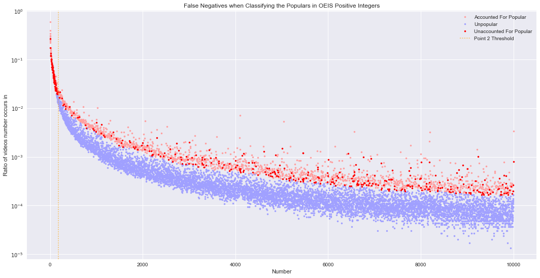
The graph below shows where the unaccounted for popular numbers fall within the OEIS popularity graph. It seems many of them occur for smaller numbers, before a clear gap begins to appear. Point 2 (from the section on classifying popular numbers) is a good marker of where a gap just starts appearing – shown as an orange dashed line in the graph (x = 185). Of the 408 unaccounted for integers, 20.1% are below point 2. Additionally, 52.9% of all popular integers below point 2 are unaccounted for. Only 1.85% of all integers are below point 2. Therefore, it seems being smaller is also an indicator for being popular.
plt.semilogy(oeis_popular_accounted.number, oeis_popular_accounted['pct'], c='#ffa0a0', marker='.', linestyle='', label='Accounted For Popular')
plt.semilogy(oeis_regular.number, oeis_regular['pct'], c='#a0a0ff', marker='.', linestyle='', label='Unpopular')
plt.semilogy(oeis_popular_unaccounted.number, oeis_popular_unaccounted['pct'], c='red', marker='.', linestyle='', label='Unaccounted For Popular')
plt.legend()
plt.xlabel('Number')
plt.ylabel('Ratio of videos number occurs in')
plt.title('False Negatives when Classifying the Populars in OEIS Positive Integers')
plt.show()

count_unaccounted_below_point2 = len([v for v in oeis_popular_unaccounted.number < point2.x if v])
count_all_popular_below_point2 = len([v for v in oeis_popular.number < point2.x if v])
print('Percent of unaccounted for below point 2: %0.2f%%' % (100 * count_unaccounted_below_point2 / len(oeis_popular_unaccounted)))
print('Percent of popular (below point 2) that are unaccounted: %0.2f%%' % (100 * count_unaccounted_below_point2 / count_all_popular_below_point2))

Percent of unaccounted for below point 2: 20.10%
Percent of popular (below point 2) that are unaccounted: 52.90%
The False Positives
We took a brief look at the numbers that should have been predicted as popular, but weren’t. Now we’ll look at the numbers that were predicted as popular, but shouldn’t be (i.e. the false positives).
oeis_predicted_popular = oeis[oeis.unionPriorWork]
oeis_true_positve = oeis_predicted_popular[oeis_predicted_popular.popular]
oeis_false_positive = oeis_predicted_popular[~oeis_predicted_popular.popular]

print("False positives: (length = {length})".format(length=len(oeis_false_positive)))
print([int(n) for n in oeis_false_positive.number])
print()

plt.semilogy(oeis_popular.number, oeis_popular['pct'], c='#ffa0a0', marker='.', linestyle='', label='Popular')
plt.semilogy(oeis_regular.number, oeis_regular['pct'], c='#a0a0ff', marker='.', linestyle='', label='Unpopular')
plt.semilogy(oeis_false_positive.number, oeis_false_positive['pct'], c='blue', marker='.', linestyle='', label='False Positives')
plt.legend()
plt.xlabel('Number')
plt.ylabel('Ratio of videos number occurs in')
plt.title('False Positives when Classifying the Populars in OEIS Positive Integers')
plt.show()
False positives: (length = 163)
[196, 243, 289, 320, 343, 361, 448, 484, 513, 529, 640, 648, 676, 704, 800, 832, 896, 947, 972, 983, 1056, 1088, 1216, 1248, 1408, 1472, 1568, 1632, 1664, 1699, 1760, 1824, 1856, 1984, 2176, 2208, 2368, 2430, 2432, 2448, 2464, 2496, 2624, 2736, 2752, 2784, 2843, 2912, 2944, 2963, 2976, 3008, 3040, 3083, 3187, 3392, 3402, 3520, 3552, 3564, 3648, 3672, 3712, 3776, 3808, 3904, 3920, 3923, 3936, 4176, 4212, 4256, 4288, 4327, 4363, 4512, 4544, 4576, 4640, 4672, 4736, 4928, 4960, 4968, 4992, 5056, 5088, 5152, 5248, 5312, 5328, 5346, 5472, 5488, 5504, 5508, 5520, 5568, 5664, 5696, 5791, 5808, 5903, 5987, 6016, 6080, 6192, 6208, 6264, 6287, 6318, 6384, 6432, 6464, 6496, 6592, 6688, 6696, 6703, 6784, 6823, 7104, 7232, 7237, 7243, 7296, 7360, 7452, 7552, 7584, 7632, 7643, 7808, 7872, 7904, 7933, 7968, 8096, 8262, 8316, 8352, 8496, 8539, 8544, 8576, 8623, 8768, 8832, 8863, 8896, 8928, 8963, 9024, 9088, 9152, 9280, 9288, 9344, 9396, 9467, 9680, 9743, 9888]

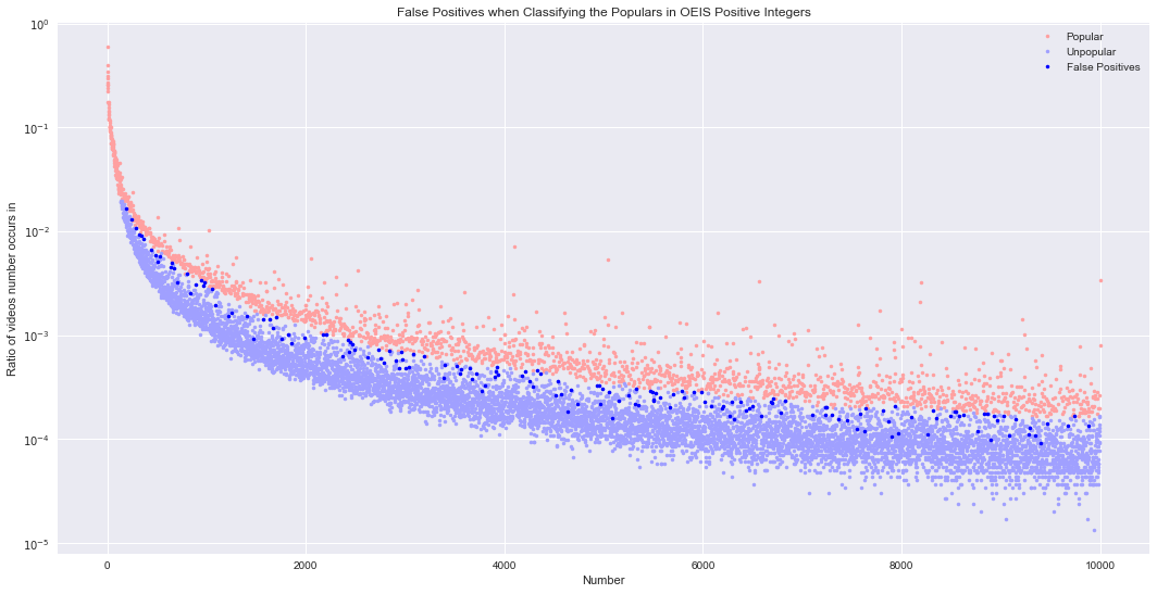
Almost all of the false positives fall within the muddy gap. There are still plenty in the muddy gap that weren’t false positives though. In the future, it might be interesting to try characterizing numbers in the muddy gap.
The Most Popular
So just who are the most popular positive integers in OEIS?
oeis_sorted = oeis.sort_values(by='pct', ascending=False)
tenth_value = oeis_sorted.iloc[9].pct
print(oeis_sorted[oeis_sorted.pct >= tenth_value][['number', 'count', 'pct']])
         number   count       pct
1000002     1.0  177633  0.599055
1000003     2.0  117126  0.394999
1000004     3.0  102140  0.344460
1000005     4.0   92043  0.310409
1000006     5.0   87105  0.293756
1000007     6.0   79892  0.269430
1000008     7.0   75694  0.255273
1000001     0.0   75597  0.254946
1000009     8.0   71019  0.239507
1000010     9.0   65758  0.221764
It turns out that the ten most popular positive integers in OEIS are zero through nine, mostly in that order – zero is wedged between seven and eight. The most popular integer is one, which is 1.5 times more popular than the second number (two). Nilsson and Hutton et al., 1969 conjectured that one was the loneliest number, with two being almost as lonely, but according to OEIS they are actually the most popular!
Featured Figures and Future Figuring
We covered a lot this time:
- We got our first glimpse of the popularity of positive rationals across the three sources, then took a deep dive into the OEIS positive integers.
- The popularity of OEIS positive integers generally follows: popularity = 12.226418 * n^-1.293657 (similar to the Sloane’s Gap paper)
- We found that being prime, a power, one off of being a power of two, being a square number, or being highly composite are all good indicators of being popular. Having relatively more prime factors than neighboring numbers can also be an indicator, but isn’t as good.
- 20.8% of popular integers don’t fall into any of those categories though. Many of them are just small, before a noticeable gap starts appearing.
- One is the most popular positive integer in OEIS
Overall, I was generally able to replicate the findings from prior work (Guglielmetti and Gauvrit et al.). Next time, I’ll venture into new territory by exploring the Numberphile positive rationals!